

The transformer is a neural network architecture that was proposed in the paper "Attention is All You Need" by Ashish Vaswani, et al. in 2017. It is a powerful architecture that lead to many state-of-the-art results in the last few years. It can be used to generate text (GPT-3), create beautiful images from text (Imagen, Dall-e 2, Stable diffusion), compose music (music transformer), speech-to-text (Whisper), understanding protein structure (AlphaFold), teaching cars to drive themselves (Tesla FSD) or even learn to do many different tasks (Gato). There are probably many amazing results I forgot to name, and many more to come.
Large language models (LLMs) are going to have a large impact in the future. We are probably going to interact with these models a lot in the future to brainstorm, help us with creativity, make sense of large amounts of information and maybe even understand ourselves better. GPT-3 is already helping me with coding and writing (also for this blogpost), and these models are going to get better really fast. That is why I want to understand how they work.
In this blogpost I will show you how to build a text generation model from scratch using the transformer architecture. I will show the coding process, and will try to make each step as simple as possible. The aim of this post is not to build the best text generation model, but to try to make each step of building one as clear as possible.
Overview
Text generation models like GPT-3 are built using the transformer architecture. This architecture was first proposed in the 2017 paper "Attention is All You Need".
Unlike typical sequence-to-sequence models used for translation tasks, which have both an encoder and decoder, text generation models only require a decoder. This is because the input and output sequences are essentially the same - the model generates text token-by-token based on previous context.
The decoder-only architecture looks like this:
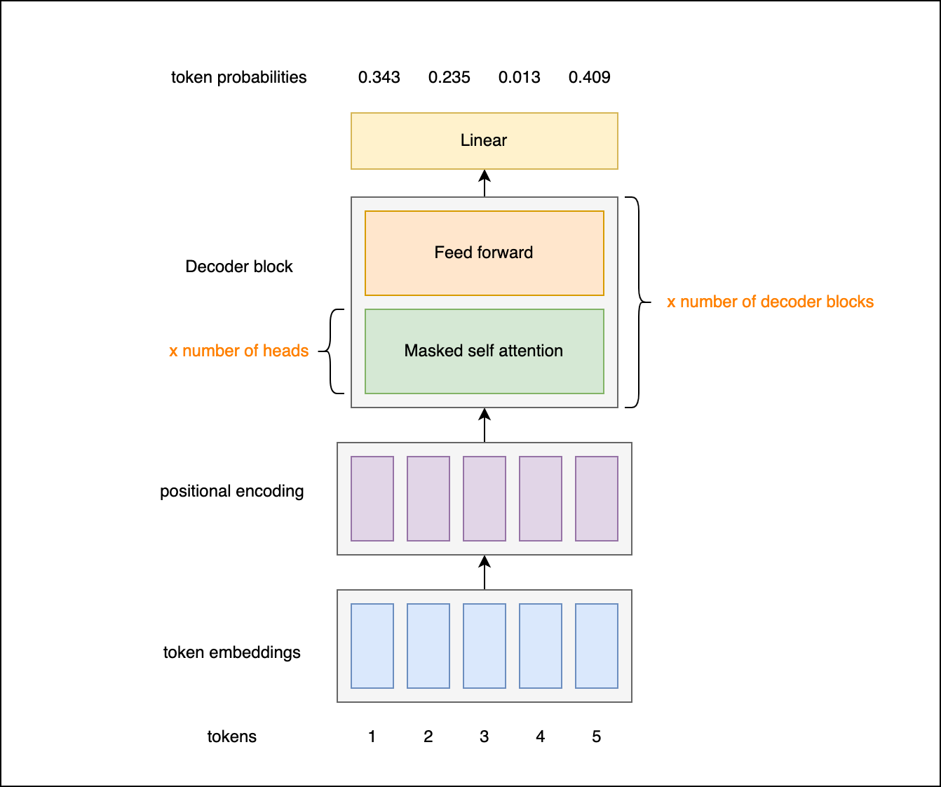
So for text generation, we only need to focus on implementing the decoder portion. The key components we'll cover are:
- Tokenization - breaking text into tokens
- Input embeddings - turning tokens into vectors
- Positional encodings - retaining sequence order information
- Masking - preventing model from peeking ahead or looking at padding tokens
- Multi-headed self-attention - relating different input tokens
- Decoder stack - refining understanding over multiple layers
- Language model head - predicting token probabilities
By incrementally implementing each of these pieces, we'll end up with a full text generation model. I'll explain both the concepts and show concrete code for each part.
The goal is to provide an intuitive understanding of how transformers work under the hood. Let's get started with tokenization!
Tokenizing the text
Natural language processing models like transformers operate on numerical data. However, our raw data is often in the form of human-readable text. To bridge this gap, we employ a process called tokenization.
Tokenization involves breaking down the text into smaller chunks known as tokens. The granularity of these tokens can range widely: a token might be as small as a single character, as large as a word, or anywhere in between. The choice of token size depends on the specific task and method being used.
For instance, GPT-3 uses a form of tokenization called Byte Pair Encoding (BPE), which tokenizes text into subwords. These subwords are sequences of characters that frequently appear together. This approach is a middle ground between character-level and word-level tokenization, balancing efficiency and versatility.
The Role of a Vocabulary
Tokenization involves converting each token in the text into a unique integer identifier, or index, using a dictionary called a vocabulary. The vocabulary consists of a list of all unique tokens that the model should recognize.
Consider the sentence "I am a cat." If our vocabulary is ["<PAD>", "I", "am", "a", "cat", "dog", "mouse"], each word in the sentence maps to an index in the vocabulary. "I" corresponds to 1, "am" to 2, "a" to 3, and "cat" to 4. So, our sentence becomes [1, 2, 3, 4] in numerical form.
Dealing with Variable-Length Inputs: Padding
Transformers typically expect inputs of a fixed size. However, real-world text data comes in sequences of variable length. To accommodate this, we use a technique called padding.
Padding involves supplementing shorter sequences with extra tokens (typically designated by the index 0) to match the length of the longest sequence in the batch. For instance, if we want all inputs to be six tokens long, our example sentence "I am a cat." becomes [0, 0, 1, 2, 3, 4].
The size of a vocabulary depends on the complexity of the language and the granularity of the tokenization. We are going to use a simple tokenizer which recognizes just 39 tokens.
On the other hand, GPT-3's tokenizer uses a vocabulary of 50,257 tokens. This large vocabulary includes a broad range of English words, common word parts, and even whole phrases, enabling GPT-3 to understand and generate highly diverse and nuanced text.
Simple tokenizer example
We create a very simple tokenizer that can encode the characters a-z, the numbers 0-9 a period and a whitespace character. The padding token is mapped to 0.
Our dictionary is very simple, and contains only 39 tokens.
class Tokenizer:

    def __init__(self):
        self.dictionary = {}
        self.reverse_dictionary = {}

        # Add the padding token
        self.__add_to_dict('<pad>')

        # Add characters and numbers to the dictionary
        for i in range(10):
            self.__add_to_dict(str(i))
        for i in range(26):
            self.__add_to_dict(chr(ord('a') + i))

        # Add space and punctuation to the dictionary
        self.__add_to_dict('.')
        self.__add_to_dict(' ')

    def __add_to_dict(self, character):
        if character not in self.dictionary:
            self.dictionary[character] = len(self.dictionary)
            self.reverse_dictionary[self.dictionary[character]] = character

    def tokenize(self, text):
        return [self.dictionary[c] for c in text]

    def character_to_token(self, character):
        return self.dictionary[character]

    def token_to_character(self, token):
        return self.reverse_dictionary[token]

    def size(self):
        return len(self.dictionary)
Dataset
Once the model and the tokenization process have been defined, the next step is preparing a suitable dataset to train the model. As we're aiming for simplicity to illustrate the process, let's construct a "hello world" equivalent dataset for text generation.
Our toy dataset will consist of simple, self-contained sentences. Each sentence communicates a fact about a particular animal, such as "cats rule the world" or "penguins live in the Arctic."
# Create the training data
training_data = '. '.join([
    'cats rule the world',
    'dogs are the best',
    'elephants have long trunks',
    'monkeys like bananas',
    'pandas eat bamboo',
    'tigers are dangerous',
    'zebras have stripes',
    'lions are the kings of the savannah',
    'giraffes have long necks',
    'hippos are big and scary',
    'rhinos have horns',
    'penguins live in the arctic',
    'polar bears are white'
])
With the raw data prepared, we can then tokenize it. This process converts each character in our training sentences into its corresponding token index from the vocabulary.
# Tokenize the training data
tokenized_training_data = tokenizer.tokenize(training_data)
Remember that our model expects input sequences of a fixed length, yet our sentences vary in length. To address this, we'll use padding, specifically left-padding.
Left-padding involves prepending padding tokens ("<pad>") to the beginning of shorter sequences until they match the length of the longest sequence in our dataset. By padding our sequences in this way, we ensure that every token in every sequence, no matter its original length, will be used in the training process.
# Left-pad the tokenized training data
for _ in range(max_sequence_length):
    # Prepend padding tokens
    tokenized_training_data.insert(0, tokenizer.character_to_token('<pad>'))
Input embedding
In textual data processing, one of the most critical steps is converting words or tokens into numerical representations that computational models can understand and work with. This transformation is performed by an embedding layer.
Imagine tokens as atomic units of meaning in a language - they can be words, parts of words, or even entire phrases. When tokenizing, we replace these units with corresponding integers. However, to effectively capture the nuances of language and the relationship between different tokens, we need to take a step further.
That's where the embedding layer comes in, acting as a bridge between discrete tokens and continuous vector space. It transforms each token, represented as an integer, into a continuous vector in a high-dimensional space.
Embeddings and Semantic Relationships
Let's consider a simplified example. If our tokens are words, the embedding layer helps capture the similarity between "cats" and "dogs" by positioning their corresponding vectors close together in the vector space. This closeness stems from the fact that "cats" and "dogs" often appear in similar contexts.
However, the magic doesn't stop there. As we stack multiple layers in our model, each subsequent layer can capture more and more complex concepts. The first layer might understand similar animals, like cats and dogs. Higher layers might recognize the roles these animals play in sentences, such as being pets. Even higher layers might comprehend more complex semantic structures, like cats and dogs representing different aspects of a shared concept (pets).
Creating an Embedding Layer with PyTorch
In PyTorch, the nn.Embedding class helps us create the embedding layer. During training, this layer's weights (representing our token embeddings) get updated and fine-tuned to better capture the semantic relationships between different tokens.
Here is a simplified code snippet illustrating the implementation of a token embedding layer:
class TokenEmbedding(torch.nn.Module):
    """
    PyTorch module that converts tokens into embeddings.

    Input dimension is: (batch_size, sequence_length)
    Output dimension is: (batch_size, sequence_length, d_model)
    """

    def __init__(self, d_model, number_of_tokens):
        super().__init__()
        self.embedding_layer = torch.nn.Embedding(
            num_embeddings=number_of_tokens,
            embedding_dim=d_model
        )

    def forward(self, x):
        return self.embedding_layer(x)
In the code above:
number_of_tokensindicates the total number of unique tokens our model can encounter in the input. This number typically equals the size of our token dictionary.d_modelspecifies the size (dimensionality) of the embedding vectors. Higher dimensions allow us to encode more information about each token, but also increase the computational complexity and the time required to train the model.
The input to our TokenEmbedding module is a batch of sequences, with each token represented by an integer. The output, in contrast, is a batch of the same sequences, but each integer is now replaced by a rich, high-dimensional vector encapsulating semantic information.
Positional encoding
Why is positional encoding necessary?
Transformers operate based on the idea of self-attention, which computes relevance scores for elements in the input sequence relative to each other. However, transformers don't inherently account for the sequence order because the self-attention mechanism treats input elements independently.
In tasks like natural language understanding, the order of elements is crucially important. For instance, the sentences "The cat chases the mouse" and "The mouse chases the cat" carry very different meanings. Without considering the positional information, a transformer might interpret these sentences as equivalent. This is why we need positional encoding – to instill a sense of sequence order into transformers.
How does positional encoding work?
In the original Transformer model, positional encoding is carried out by creating a vector for each position in the sequence and adding it to the corresponding input vector. This is done so the model can learn to utilize these position vectors to understand the order of elements in the sequence.
Specifically, the positional encoding for a position "p" and dimension "i" in the input sequence is computed using these sine and cosine functions:
PE(p, 2i) = sin(p / 10000^(2i/d_model))
PE(p, 2i+1) = cos(p / 10000^(2i/d_model))
Here, "d_model" is the dimensionality of the input and output vectors in the model. A larger "d_model" would mean that each word is represented by a larger vector, allowing for more complex representations but also requiring more computational resources. The sin and cos functions are applied alternately to each dimension of the positional encoding vector, creating a pattern that the model can learn and recognize.
The resulting positional encodings vary between -1 and 1, and they have a wavelength that increases with each dimension. This pattern allows the model to distinguish different positions and to generalize to sequence lengths not encountered during training.
These positional encodings are added to the input embeddings before being processed by the transformer. This allows the transformer to learn to utilize this positional information in a way that best suits the task it's being trained on. For example, the model might learn to pay more attention to adjacent words in sentence interpretation, capturing the notion that in many languages, nearby words often have a higher syntactic and semantic relevance to each other.
The code to create a module that creates and adds such a positional embedding could be written as follows:
class PositionalEncoding(torch.nn.Module):
    """
    Pytorch module that creates a positional encoding matrix. This matrix will later be added to the
    transformer's input embeddings to provide a sense of position of the sequence elements.
    """

    def __init__(self, d_model, max_sequence_length):
        super().__init__()
        self.d_model = d_model
        self.max_sequence_length = max_sequence_length
        self.positional_encoding = self.create_positional_encoding()

    def create_positional_encoding(self):
        """
        Creates a positional encoding matrix of size (max_sequence_length, d_model).
        """

        # Initialize positional encoding matrix
        positional_encoding = np.zeros((self.max_sequence_length, self.d_model))

        # Calculate positional encoding for each position and each dimension
        for pos in range(self.max_sequence_length):
            for i in range(0, self.d_model, 2):
                # Apply sin to even indices in the array; indices in Python start at 0 so i is even.
                positional_encoding[pos, i] = np.sin(pos / (10000 ** ((2 * i) / self.d_model)))

                if i + 1 < self.d_model:
                    # Apply cos to odd indices in the array; we add 1 to i because indices in Python start at 0.
                    positional_encoding[pos, i + 1] = np.cos(pos / (10000 ** ((2 * i) / self.d_model)))

        # Convert numpy array to PyTorch tensor and return it
        return torch.from_numpy(positional_encoding).float()

    def forward(self, x):
        """
        Adds the positional encoding to the input embeddings at the corresponding positions.
        """
        # Add positional encodings to input embeddings. The ":" indexing ensures we only add positional encodings up
        # to the length of the sequence in the batch. x.size(0) is the batch size, so this is a way to make sure
        # we're not adding extra positional encodings.
        return x + self.positional_encoding[:x.size(1), :]
Masking
Remember the padding tokens we talked about before? These padding tokens don't carry any information, and it's important for the model not to pay attention to them when it's processing input data.
This is where masking comes in. A mask is typically an array that has the same length as the sentence, with ones at positions corresponding to actual words and zeros at positions corresponding to the padding tokens.
When computing attention scores, we do not want to include the effect of padding tokens. To avoid this, we can apply the mask to the attention scores matrix, effectively setting the scores at padding positions to a very large negative number (e.g., -1e9). The reason for using such a large negative number is that these scores are passed through a softmax function, which will transform these large negative numbers into zeros. This means that the padding positions will not have any influence on the final output of the attention layer.
Here is a snippet of the mask application part from the MaskedSelfAttention class:
# Apply the mask to the attention weights, by setting the masked tokens to a very low value.
# This will make the softmax output 0 for these values.
mask = mask.reshape(attention_weights.shape[0], 1, attention_weights.shape[2])
attention_weights = attention_weights.masked_fill(mask == 0, -1e9)
This line is essentially applying the mask to the attention_weights tensor. The masked_fill(mask == 0, -1e9) operation is saying "for every position in attention_weights where the corresponding position in mask is zero (i.e., a padding token), replace the attention_weights value with -1e9". This ensures that padding tokens receive no attention whatsoever.
Ideally, while predicting each new word, the decoder should only have access to the words that came before it in the sequence, not those that come after. Why? Because in real-world application, like translating a sentence, we don't have future information. The process is carried out word by word from start to end. This is known as the autoregressive property: the prediction at a certain time step depends only on the inputs and outputs at previous time steps.
To enforce this property while training the model, we use a mechanism called a causal mask (also known as a subsequent mask). This mask ensures that, for any given word, the model cannot attend to (or "peek at") the words that come after it.
Let's use an actual sentence to visualize this: "The cat sat on the mat."
If the model is trying to predict the word at the fourth position ("on"), it should only consider "The", "cat", and "sat". It should not have access to "the" or "mat". The causal mask helps us achieve this by masking out (or hiding) the future words while the model is making its prediction.
We implement this using torch.tril to create a lower-triangular matrix of ones. This ensures that position i can only attend to positions 0 through i:
# Apply causal mask to prevent attending to future positions.
# This is essential for autoregressive generation.
seq_length = x.size(1)
causal_mask = torch.tril(torch.ones(seq_length, seq_length, device=x.device)).bool()
attention_weights = attention_weights.masked_fill(~causal_mask, -1e9)
Attention
The attention mechanisms play a vital role in the transformer architecture. They're effectively a way to highlight the important parts of an input sequence, similar to how we humans pay more attention to specific parts of a sentence or image depending on the context.
Imagine we have the sentence: "The man ate a sandwich he prepared in the morning. It was topped with cheese". If we wish to understand what "It" refers to, we would naturally pay more attention to "sandwich", making it get a higher attention score. This is essentially what the attention mechanism does, calculating an attention score for each word considering all other words in the sentence.
Attention scores are derived using query, key, and value vectors. These vectors are created by multiplying the input embeddings with learned matrices (essentially a linear transformation). These vectors help calculate the attention scores, determining the impact of one token on another.
The query, key and value vectors are then used to calculate the attention scores like in the diagram below
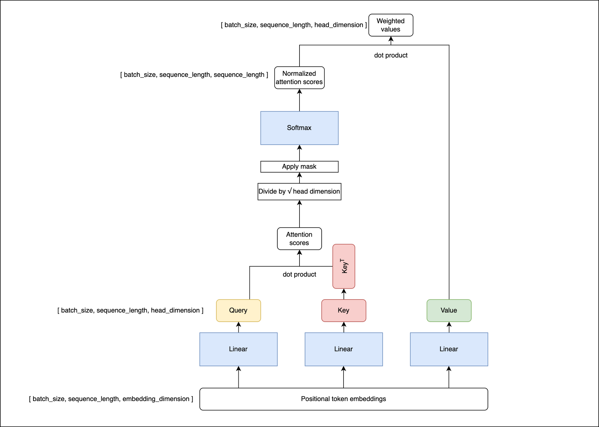
The attention scores for the tokens are calculated as the dot product between the query and key vectors. These scores are then scaled down by dividing by the square root of the query/key/value dimension (a trick from the original Transformer paper for more stable gradients).
It's important to note that attention can be masked. For masked positions, the attention score will be set to -infinity, making these positions virtually non-existent in subsequent computations.
Finally, the attention scores are normalized using the softmax function to make them fall between 0 and 1 and sum up to 1. The normalized attention scores are then multiplied with the value vectors and summed to obtain the output of the attention layer.
In PyTorch, this is how a basic attention layer would look:
class MaskedSelfAttention(torch.nn.Module):
    """
    Pytorch module for a self attention layer.
    This layer is used in the MultiHeadedSelfAttention module.

    Input dimension is: (batch_size, sequence_length, embedding_dimension)
    Output dimension is: (batch_size, sequence_length, head_dimension)
    """

    def __init__(self, embedding_dimension, head_dimension):
        super().__init__()
        self.embedding_dimension = embedding_dimension
        self.head_dimension = head_dimension
        self.query_layer = torch.nn.Linear(embedding_dimension, self.head_dimension)
        self.key_layer = torch.nn.Linear(embedding_dimension, self.head_dimension)
        self.value_layer = torch.nn.Linear(embedding_dimension, self.head_dimension)
        self.softmax = torch.nn.Softmax(dim=-1)

    def forward(self, x, mask):
        """
        Compute the self attention.

        x dimension is: (batch_size, sequence_length, embedding_dimension)
        output dimension is: (batch_size, sequence_length, head_dimension)
        mask dimension is: (batch_size, sequence_length)

        mask values are: 0 or 1. 0 means the token is masked, 1 means the token is not masked.
        """

        # x dimensions are: (batch_size, sequence_length, embedding_dimension)
        # query, key, value dimensions are: (batch_size, sequence_length, head_dimension)
        query = self.query_layer(x)
        key = self.key_layer(x)
        value = self.value_layer(x)

        # Calculate the attention weights.
        # attention_weights dimensions are: (batch_size, sequence_length, sequence_length)
        attention_weights = torch.matmul(query, key.transpose(-2, -1))

        # Scale the attention weights.
        attention_weights = attention_weights / np.sqrt(self.head_dimension)

        # Apply the mask to the attention weights, by setting the masked tokens to a very low value.
        # This will make the softmax output 0 for these values.
        mask = mask.reshape(attention_weights.shape[0], 1, attention_weights.shape[2])
        attention_weights = attention_weights.masked_fill(mask == 0, -1e9)

        # Softmax makes sure all scores are between 0 and 1 and the sum of scores is 1.
        # attention_scores dimensions are: (batch_size, sequence_length, sequence_length)
        attention_scores = self.softmax(attention_weights)

        # The attention scores are multiplied by the value
        # Values of tokens with high attention score get highlighted because they are multiplied by a larger number,
        # and tokens with low attention score get drowned out because they are multiplied by a smaller number.
        # Output dimensions are: (batch_size, sequence_length, head_dimension)
        return torch.bmm(attention_scores, value)
Multi-head Attention for Diverse Perspectives
The attention mechanism, as we've discussed, allows a model to focus on different parts of the input sequence when generating each word in the output sequence. But there's an additional refinement we can make to this system to make it even more powerful. Instead of having one single "attention perspective", why not have multiple? That's the idea behind multi-head attention.
Imagine a class of students all looking at the same picture, but each student noticing and focusing on different details — one might notice the colors, another the shapes, another the overall composition. They each bring their own unique "perspective" to understanding the picture as a whole.
The Transformer model does something similar with multi-head attention. It has not one, but multiple sets (or "heads") of the attention mechanism, each of which independently focuses on different parts of the input. Each head can learn to pay attention to different positions of the input sequence and extract different types of information. For example, one attention head might learn to focus on syntactic aspects of the language (like grammar), while another might learn semantic information (like meaning).
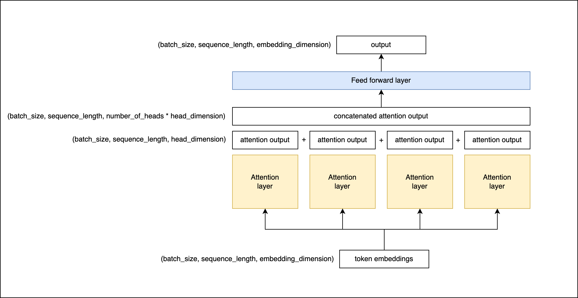
Here is how it works:
Each head computes its own query, key, and value matrices from the input, just like in the single-head attention mechanism. They then compute their attention scores and produce an output. But instead of being processed individually, the output of each head is concatenated together and then transformed with a linear layer to produce the final output.
This is the code for the MaskedMultiHeadedSelfAttention class:
class MaskedMultiHeadedSelfAttention(torch.nn.Module):
    """
    Pytorch module for a multi head attention layer.

    Input dimension is: (batch_size, sequence_length, embedding_dimension)
    Output dimension is: (batch_size, sequence_length, embedding_dimension)
    """

    def __init__(self, embedding_dimension, number_of_heads):
        super().__init__()
        self.embedding_dimension = embedding_dimension
        self.head_dimension = embedding_dimension // number_of_heads
        self.number_of_heads = number_of_heads

        # Create the self attention modules
        self.self_attentions = torch.nn.ModuleList(
            [MaskedSelfAttention(embedding_dimension, self.head_dimension) for _ in range(number_of_heads)])

        # Create a linear layer to combine the outputs of the self attention modules
        self.output_layer = torch.nn.Linear(number_of_heads * self.head_dimension, embedding_dimension)

    def forward(self, x, mask):
        """
        Compute the multi head attention.

        x dimensions are: (batch_size, sequence_length, embedding_dimension)
        mask dimensions are: (batch_size, sequence_length)
        mask values are: 0 or 1. 0 means the token is masked, 1 means the token is not masked.
        """
        # Compute the self attention for each head
        # self_attention_outputs dimensions are:
        # (number_of_heads, batch_size, sequence_length, head_dimension)
        self_attention_outputs = [self_attention(x, mask) for self_attention in self.self_attentions]

        # Concatenate the self attention outputs
        # self_attention_outputs_concatenated dimensions are:
        # (batch_size, sequence_length, number_of_heads * head_dimension)
        concatenated_self_attention_outputs = torch.cat(self_attention_outputs, dim=2)

        # Apply the output layer to the concatenated self attention outputs
        # output dimensions are: (batch_size, sequence_length, embedding_dimension)
        return self.output_layer(concatenated_self_attention_outputs)
The decoder layer
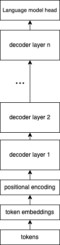
The model consists of several decoder layer. Each decoder takes the output of the previous decoder as input. The first decoder takes the positional encoding layer as input. The final layer is a language model head, which is going to output the probabilies of next tokens.
In the case of an autoregressive model like GPT-2, each decoder layer is composed of a self-attention mechanism and a feed-forward neural network. The self-attention mechanism allows the model to weigh the importance of different tokens in the input when predicting the next token, while the feed-forward network enables the model to learn more traditional, positional relationships between the tokens.
When we stack multiple of these decoder layers on top of each other, it allows the model to refine its understanding of the input data over several rounds of processing. The output of one layer becomes the input of the next, and so the model can use the output of previous layers to inform its understanding of the current layer. Each layer can learn to represent different features or aspects of the input data. The higher-level layers (further in the stack) can capture more complex or abstract features, which are compositions of the simpler features captured by the lower-level layers (earlier in the stack).
So, in essence, the stacking of multiple decoder layers enables the model to capture more complex patterns and understand deeper contextual relationships among the data, thereby resulting in more accurate predictions.
So, what does each decoder layer do exactly?
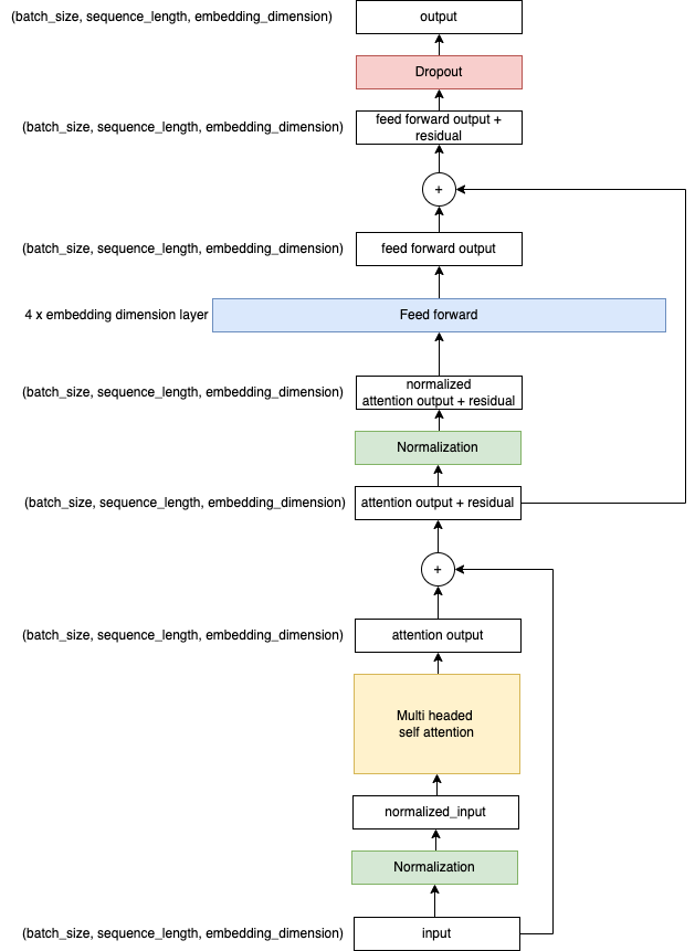
Step 1: Input and Layer Normalization
When a decoder layer receives its input, the very first thing it does is apply layer normalization to these input vectors. The inputs to the decoder are high-dimensional vectors that each represent a token in the sequence.
Layer normalization is a crucial process that ensures the numerical stability of the model. It prevents numbers from getting too large during training, mitigating what's known as the "exploding gradients" problem.
But layer normalization does more than just guard against large numbers. It helps spread the data more evenly throughout the feature space, which makes the learning process more effective. By adjusting the embeddings such that each dimension has a mean of 0 and a standard deviation of 1, it ensures that no particular feature has undue influence over others due to differences in scale. This equalization of influence across dimensions is key for a balanced and efficient learning process.
Step 2: Self-Attention
Once the inputs are normalized, the decoder layer applies the self-attention mechanism. This allows the model to weigh the importance of each token in the sequence relative to the others, providing a context-aware representation of each token.
Step 3: Residual Connections
The output from the self-attention process is then added to the original input (before normalization) in what's known as a residual connection. This connection is a clever way of allowing the gradients to flow directly through the network, mitigating another common deep learning problem: vanishing gradients. The "vanishing gradients" problem refers to gradients getting exponentially smaller as they propagate back through the layers during training, making it harder for the model to learn and adjust its earlier layers.
Step 4: Another Round of Normalization and Feed-Forward Network
After applying the residual connection, the output is normalized once again and then passed through a feed-forward neural network. This network is a fully connected layer that applies non-linear transformations (like ReLU) to the data, allowing the model to learn complex relationships in the data.
Step 5: Dropout
Finally, to prevent overfitting to the training data, a dropout procedure is applied. This process randomly drops out (i.e., temporarily removes during training, 10% in my example code) a percentage of the connections in the model. In this way, it encourages the model to learn a more robust representation of the data that doesn't rely too heavily on any single connection.
After going through all these steps, the output of one decoder layer becomes the input to the next. This stacking of multiple decoders allows the model to learn to represent the data at various levels of abstraction, which is key to its ability to understand and generate human-like text.
The entire process of the decoder layer can be seen in code through the DecoderLayer and DecoderStack classes, where DecoderLayer encapsulates the processes within a single layer, and DecoderStack handles the stacking of multiple DecoderLayers.
class DecoderLayer(torch.nn.Module):
    """
    Pytorch module for an encoder layer.

    An encoder layer consists of a multi-headed self attention layer, a feed forward layer and dropout.

    Input dimension is: (batch_size, sequence_length, embedding_dimension)
    Output dimension is: (batch_size, sequence_length, embedding_dimension)
    """

    def __init__(
            self,
            embedding_dimension,
            number_of_heads,
            feed_forward_dimension,
            dropout_rate
    ):
        super().__init__()
        self.embedding_dimension = embedding_dimension
        self.number_of_heads = number_of_heads
        self.feed_forward_dimension = feed_forward_dimension
        self.dropout_rate = dropout_rate

        self.multi_headed_self_attention = MaskedMultiHeadedSelfAttention(embedding_dimension, number_of_heads)
        self.feed_forward = FeedForward(embedding_dimension, feed_forward_dimension)
        self.dropout = torch.nn.Dropout(dropout_rate)
        self.layer_normalization_1 = torch.nn.LayerNorm(embedding_dimension)
        self.layer_normalization_2 = torch.nn.LayerNorm(embedding_dimension)

    def forward(self, x, mask):
        """
        Compute the encoder layer.

        x dimensions are: (batch_size, sequence_length, embedding_dimension)
        mask dimensions are: (batch_size, sequence_length)
        mask values are: 0 or 1. 0 means the token is masked, 1 means the token is not masked.
        """

        # Layer normalization 1
        normalized_x = self.layer_normalization_1(x)

        # Multi headed self attention
        attention_output = self.multi_headed_self_attention(normalized_x, mask)

        # Residual output
        residual_output = x + attention_output

        # Layer normalization 2
        normalized_residual_output = self.layer_normalization_2(residual_output)

        # Feed forward
        feed_forward_output = self.feed_forward(normalized_residual_output)

        # Dropout, only when training.
        if self.training:
            feed_forward_output = self.dropout(feed_forward_output)

        # Residual output
        return residual_output + feed_forward_output
The DecoderStack is a number of decoder layers in sequence.
class DecoderStack(torch.nn.Module):
    """
    Pytorch module for a stack of decoders.
    """

    def __init__(
            self,
            embedding_dimension,
            number_of_layers,
            number_of_heads,
            feed_forward_dimension,
            dropout_rate,
            max_sequence_length
    ):
        super().__init__()
        self.embedding_dimension = embedding_dimension
        self.number_of_layers = number_of_layers
        self.number_of_heads = number_of_heads
        self.feed_forward_dimension = feed_forward_dimension
        self.dropout_rate = dropout_rate
        self.max_sequence_length = max_sequence_length

        # Create the encoder layers
        self.encoder_layers = torch.nn.ModuleList(
            [DecoderLayer(embedding_dimension, number_of_heads, feed_forward_dimension, dropout_rate) for _ in
             range(number_of_layers)])

    def forward(self, x, mask):
        decoder_outputs = x
        for decoder_layer in self.encoder_layers:
            decoder_outputs = decoder_layer(decoder_outputs, mask)

        return decoder_outputs
The feed forward layer
class FeedForward(torch.nn.Module):
    """
    Pytorch module for a feed forward layer.

    A feed forward layer is a fully connected layer with a ReLU activation function in between.
    """

    def __init__(self, embedding_dimension, feed_forward_dimension):
        super().__init__()
        self.embedding_dimension = embedding_dimension
        self.feed_forward_dimension = feed_forward_dimension
        self.linear_1 = torch.nn.Linear(embedding_dimension, feed_forward_dimension)
        self.linear_2 = torch.nn.Linear(feed_forward_dimension, embedding_dimension)

    def forward(self, x):
        """
        Compute the feed forward layer.
        """
        return self.linear_2(torch.relu(self.linear_1(x)))
The model
the LanguageModel class brings together all the layers we've discussed so far: token embeddings, positional encoding, normalization, and the decoder stack. Let's go through each component:
- Token Embedding: The model first creates token embeddings. Each token (word, subword, or character) in the input sequence is represented by a high-dimensional vector, which is initialized randomly and learned during training. The embedding dimension is a hyperparameter.
- Positional Encoding: The model then applies positional encoding to the token embeddings. This helps the model to understand the order of the tokens in the sequence, a crucial piece of information in many natural language tasks. In GPT, positional encoding is achieved by adding a vector to each token embedding, which encodes the token's position in the sequence.
- Layer Normalization: Next, the model applies layer normalization to the result of the positional encoding. This normalization process adjusts the vectors so that each dimension has a mean of 0 and a standard deviation of 1, equalizing the influence of each dimension and helping to stabilize the learning process.
- Decoder Stack: The normalized output is then passed into a stack of decoders. Each decoder block in the stack consists of a self-attention mechanism and a feed-forward neural network, with layer normalization and residual connections used throughout.
After the data passes through the decoder stack, we reach the final part of the model: the language model head.
class LanguageModel(torch.nn.Module):
    """
    Pytorch module for a language model.
    """

    def __init__(
            self,
            number_of_tokens,  # The number of tokens in the vocabulary
            max_sequence_length=512,  # The maximum sequence length to use for attention
            embedding_dimension=512,  # The dimension of the token embeddings
            number_of_layers=6,  # The number of decoder layers to use
            number_of_heads=4,  # The number of attention heads to use
            feed_forward_dimension=None,  # The dimension of the feed forward layer
            dropout_rate=0.1  # The dropout rate to use
    ):
        super().__init__()
        self.number_of_tokens = number_of_tokens
        self.max_sequence_length = max_sequence_length
        self.embedding_dimension = embedding_dimension
        self.number_of_layers = number_of_layers
        self.number_of_heads = number_of_heads

        if feed_forward_dimension is None:
            # GPT-2 paper uses 4 * embedding_dimension for the feed forward dimension
            self.feed_forward_dimension = embedding_dimension * 4
        else:
            self.feed_forward_dimension = feed_forward_dimension

        self.dropout_rate = dropout_rate

        # Create the token embedding layer
        self.token_embedding = TokenEmbedding(embedding_dimension, number_of_tokens)

        # Create the positional encoding layer
        self.positional_encoding = PositionalEncoding(embedding_dimension, max_sequence_length)

        # Create the normalization layer
        self.layer_normalization = torch.nn.LayerNorm(embedding_dimension)

        # Create the decoder stack
        self.decoder = DecoderStack(
            embedding_dimension=embedding_dimension,
            number_of_layers=number_of_layers,
            number_of_heads=number_of_heads,
            feed_forward_dimension=self.feed_forward_dimension,
            dropout_rate=dropout_rate,
            max_sequence_length=max_sequence_length
        )

        # Create the language model head
        self.lm_head = LMHead(embedding_dimension, number_of_tokens)

    def forward(self, x, mask):
        # Compute the token embeddings
        # token_embeddings dimensions are: (batch_size, sequence_length, embedding_dimension)
        token_embeddings = self.token_embedding(x)

        # Compute the positional encoding
        # positional_encoding dimensions are: (batch_size, sequence_length, embedding_dimension)
        positional_encoding = self.positional_encoding(token_embeddings)

        # Post embedding layer normalization
        positional_encoding_normalized = self.layer_normalization(positional_encoding)

        decoder_outputs = self.decoder(positional_encoding_normalized, mask)
        lm_head_outputs = self.lm_head(decoder_outputs)

        return lm_head_outputs
Language Model Head
The LanguageModel class concludes with the LMHead layer. This layer is essentially a linear transformation that maps the high-dimensional output of the decoder stack back down to the dimension of the token vocabulary.
To put it in simpler terms, imagine you have a vocabulary of 10,000 unique words and your decoder's output dimension is 512. Each word in your vocabulary is going to have a unique 512-dimensional vector representation after passing through the decoder. But we want to assign a probability to each word in the vocabulary given the preceding context. This is where LMHead comes in.
LMHead maps the 512-dimensional vector back to the 10,000-dimensional space, essentially assigning a score to each of the 10,000 words. These scores are then passed through a softmax function to convert them into probabilities. Therefore, LMHead is crucial in transforming the high-dimensional output of the decoder stack to the likelihood of each word being the next word in the sequence.
The LMHead is implemented as a subclass of PyTorch's torch.nn.Module. It uses a linear layer (a basic type of neural network layer that applies a linear transformation to the input) to map the decoder's output dimension to the number of tokens in the vocabulary.
Consider a scenario where the model has processed the phrase "The quick brown fox". The decoder stack outputs a 512-dimensional vector for the final word "fox".
Now, let's imagine our vocabulary consists of just five words: "jumps", "sleeps", "eats", "runs", and "fox". We want to determine the likelihood of each of these words being the next word in the sentence.
That's where the LMHead comes into play. This linear layer maps the 512-dimensional vector to a 5-dimensional vector, since we have 5 words in our vocabulary. Each entry in this output vector corresponds to a word in the vocabulary, and can be interpreted as a raw score for how likely that word is to follow the phrase "The quick brown fox".
Assume the probabilities after applying softmax are: ["jumps": 0.6, "sleeps": 0.05, "eats": 0.2, "runs": 0.13, "fox": 0.02]. So the model predicts "The quick brown fox jumps" as the most likely continuation of the input sequence.
class LMHead(torch.nn.Module):
    """
    Pytorch module for the language model head.
    The language model head is a linear layer that maps the embedding dimension to the vocabulary size.
    """

    def __init__(self, embedding_dimension, number_of_tokens):
        super().__init__()
        self.embedding_dimension = embedding_dimension
        self.number_of_tokens = number_of_tokens
        self.linear = torch.nn.Linear(embedding_dimension, number_of_tokens)

    def forward(self, x):
        """
        Compute the language model head.

        x dimensions are: (batch_size, sequence_length, embedding_dimension)
        output dimensions are: (batch_size, sequence_length, number_of_tokens)
        """
        # Compute the linear layer
        # linear_output dimensions are: (batch_size, sequence_length, number_of_tokens)
        linear_output = self.linear(x)

        return linear_output
Autoregressive Wrapper
To allow our language model to generate text one token at a time, we wrap it in an autoregressive module. In an autoregressive model, the output from previous steps is fed as input to subsequent steps. This is where the AutoregressiveWrapper comes in.
The autoregressive wrapper takes a sequence of tokens as input, where the sequence length is one token more than the maximum sequence length allowed. This extra token is necessary because in autoregressive models, the model is trained to predict the next token in the sequence given the previous tokens.
For instance, consider the sentence: "The cat sat on the mat". If the input sequence is "The cat sat on the", the target output sequence (the sequence that the model is trained to predict) is "cat sat on the mat". This is why the input sequence is shifted one step to the left relative to the output sequence.
The AutoregressiveWrapper class also includes a method for calculating the probabilities of the next token in the sequence. It generates these probabilities by applying a softmax function to the logits (the raw, unnormalized scores output by the model for each token in the vocabulary) associated with the last token in the sequence. A "temperature" parameter is used to adjust the sharpness of the probability distribution. Lower temperatures make the output more deterministic (i.e., more likely to choose the most probable token), while higher temperatures make the output more random.
class AutoregressiveWrapper(torch.nn.Module):
    """
    Pytorch module that wraps a GPT model and makes it autoregressive.
    """

    def __init__(self, gpt_model):
        super().__init__()
        self.model = gpt_model
        self.max_sequence_length = self.model.max_sequence_length

    def forward(self, x, mask):
        """
        Autoregressive forward pass
        """
        inp, target = x[:, :-1], x[:, 1:]
        mask = mask[:, :-1]

        output = self.model(inp, mask)
        return output, target

    def next_token_probabilities(self, x, mask, temperature=1.0):
        """
        Calculate the token probabilities for the next token in the sequence.
        """
        logits = self.model(x, mask)[:, -1]

        # Apply the temperature
        if temperature != 1.0:
            logits = logits / temperature

        # Apply the softmax
        probabilities = torch.softmax(logits, dim=-1)

        return probabilities
Trainer
Now we have a model that can learn how language works we need to actually train it to do so.
First we create the tokenizer, so we can convert our dataset to tokens.
Then we create the autoregressive language model. Because the dataset is very small I am going to only set a max_sequence_length of 20, but a more normal value would be 512.
I will then split the training text into sequences of [max_sequence_length + 1]. To make sure the starting tokens are also considered the data will be padded on the left.
Then we are going to train the model for 100 epochs, with a batch size of 8. An epoch means a complete pass over the training data. Batch size means that in every forward pass through the model we consider 8 sequences from the training data simultaneously. The higher the batch size the better the model can learn patterns in the data, but a higher batch size also leads to more memory usage.
def create_training_sequences(max_sequence_length, tokenized_training_data):
    # Create sequences of length max_sequence_length + 1
    # The last token of each sequence is the target token
    sequences = []
    for i in range(0, len(tokenized_training_data) - max_sequence_length - 1):
        sequences.append(tokenized_training_data[i: i + max_sequence_length + 1])
    return sequences


def tokenize_and_pad_training_data(max_sequence_length, tokenizer, training_data):
    # Tokenize the training data
    tokenized_training_data = tokenizer.tokenize(training_data)
    for _ in range(max_sequence_length):
        # Prepend padding tokens
        tokenized_training_data.insert(0, tokenizer.character_to_token('<pad>'))
    return tokenized_training_data


tokenizer = Tokenizer()

embedding_dimension = 256
max_sequence_length = 20
number_of_tokens = tokenizer.size()

# Create the model
model = AutoregressiveWrapper(LanguageModel(
    embedding_dimension=embedding_dimension,
    number_of_tokens=number_of_tokens,
    number_of_heads=4,
    number_of_layers=3,
    dropout_rate=0.1,
    max_sequence_length=max_sequence_length
))

# Create the training data
training_data = '. '.join([
    'cats rule the world',
    'dogs are the best',
    'elephants have long trunks',
    'monkeys like bananas',
    'pandas eat bamboo',
    'tigers are dangerous',
    'zebras have stripes',
    'lions are the kings of the savannah',
    'giraffes have long necks',
    'hippos are big and scary',
    'rhinos have horns',
    'penguins live in the arctic',
    'polar bears are white'
])

tokenized_and_padded_training_data = tokenize_and_pad_training_data(max_sequence_length, tokenizer, training_data)
sequences = create_training_sequences(max_sequence_length, tokenized_and_padded_training_data)

# Train the model
optimizer = torch.optim.Adam(model.parameters(), lr=0.0001)
trainer = Trainer(model, tokenizer, optimizer)
trainer.train(sequences, epochs=100, batch_size=8)
The trainer is a helper class that loops over the epochs and shuffles the data at the start of each epoch. The reason to do this is to prevent the batches from being the same every time, causing the model to overfit to these specific batches.
While creating batches we also determine the mask. All padding tokens are masked, meaning they will not be considered in the attention step.
Then we do a forward pass through the model with a batch. This means we let the model make predictions using the given data. The predictions are then compared to a target value, which is the sequence shifted by 1 step so the next token becomes visible. The model outputs probabilities for what token should be the next. The loss function knows what the answer should be. The further from its target the prediction was the higher the loss value will be.
When the loss value is calculated the model can be updated. This is done by calculating gradients; the direction the weights should be adjusted to improve the prediction of the model. The model is then slightly adjusted in the direction of the gradients, and a new batch can be processed.
If everything works as planned, the loss should go down over time. I return the loss per epoch, so it can be plotted.
class Trainer:

    def __init__(self, model, tokenizer: Tokenizer, optimizer=None):
        super().__init__()
        self.model = model
        if optimizer is None:
            self.optimizer = torch.optim.Adam(model.parameters(), lr=0.0001)
        else:
            self.optimizer = optimizer
        self.tokenizer = tokenizer
        self.loss_function = torch.nn.CrossEntropyLoss()

    def train(self, data: List[str], epochs, batch_size):
        loss_per_epoch = []
        for epoch in range(epochs):
            losses = []

            # Shuffle the sequences
            random.shuffle(data)

            # Create batches of sequences and their respective mask.
            batches = []
            for i in range(0, len(data), batch_size):
                sequence_tensor = torch.tensor(data[i: i + batch_size], dtype=torch.long)

                # Create the mask tensor for the batch, where 1 means the token is not a padding token
                mask_tensor = torch.ones_like(sequence_tensor)
                mask_tensor[sequence_tensor == self.tokenizer.character_to_token('<pad>')] = 0

                batches.append((sequence_tensor, mask_tensor))

            # Train the model on each batch
            for batch in batches:
                self.model.train()

                # Create the input and mask tensors
                input_tensor = torch.zeros((batch_size, self.model.max_sequence_length + 1), dtype=torch.long)
                mask_tensor = torch.zeros((batch_size, self.model.max_sequence_length + 1), dtype=torch.long)

                for i, input_entry in enumerate(batch[0]):
                    input_tensor[i] = input_entry

                for i, mask_entry in enumerate(batch[1]):
                    mask_tensor[i] = mask_entry

                # Compute the model output
                model_output, target = self.model.forward(x=input_tensor, mask=mask_tensor)

                # Compute the losses
                # The loss is computed on the model output and the target
                loss = self.loss_function(model_output.transpose(1, 2), target)

                # Backpropagate the loss.
                loss.backward()

                # Clip the gradients. This is used to prevent exploding gradients.
                torch.nn.utils.clip_grad_norm_(self.model.parameters(), 0.5)

                # Update the model parameters. This is done by taking a step in the direction of the gradient.
                self.optimizer.step()

                # Reset the gradients. This is done so that the gradients from the previous batch
                # are not used in the next step.
                self.optimizer.zero_grad()

                # Append the loss to the list of losses, so that the average loss can be computed for this epoch.
                losses.append(loss.item())

            # Print the loss
            epoch_loss = np.average(losses)
            loss_per_epoch.append(epoch_loss)
            print('Epoch:', epoch, 'Loss:', epoch_loss)

        return loss_per_epoch
Evenutally plotting the loss should give us a nice graph with decreasing loss. It is plotted in log scale, so you can see the smaller variations towards the end of training.
# Plot the loss per epoch in log scale
plt.plot(loss_per_epoch)
plt.yscale('log')
plt.ylabel('Loss')
plt.xlabel('Epoch')
plt.show()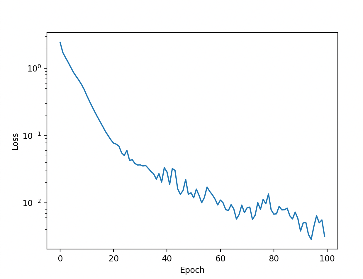
Generator
Now the model is trained and I want to see if it actually learned to write. Let's try to generate a text based on the prompt "elephants". I want it to continue writing for 50 tokens.
Since the only mention of elephants in the training data is "elephants have long trunks", I expect the model to write this.
max_tokens_to_generate = 50
generator = Generator(model, tokenizer)
generated_text = generator.generate(
    max_tokens_to_generate=max_tokens_to_generate,
    prompt="elephants",
    padding_token=tokenizer.character_to_token('<pad>')
)
print(generated_text.replace('<pad>', ''))
but first we need to write the code for the Generator. A helper class for generating text.
First we switch the model from 'training' mode to 'eval' mode. In eval mode the model will not apply dropout. We also wrap the generation in torch.no_grad() to disable gradient computation, which saves memory during inference.
The prompt we give is converted to tokens, and then padded so it has the correct sequence length.
Then we are going to auto-regressively generate new tokens and add them to the input sequence. After a token is added we run the new input sequence with the extra token through the model again, and we append a new token. We continue this process until the maximum number of characters we wanted to generate is reached, or until we have generated the eos_token, or end of sequence token. This is a token that can be defined by the user as an indication that we need to stop generating.
def pad_left(sequence, final_length, padding_token):
    return [padding_token] * (final_length - len(sequence)) + sequence


class Generator:

    def __init__(
            self,
            model,
            tokenizer):
        self.model = model
        self.tokenizer = tokenizer

    def generate(
            self,
            max_tokens_to_generate: int,
            prompt: str = None,
            temperature: float = 1.0,
            eos_token: int = None,
            padding_token: int = 0):

        self.model.eval()

        if prompt is None:
            start_tokens = [self.tokenizer.character_to_token(padding_token)]
        else:
            start_tokens = self.tokenizer.tokenize(prompt)

        input_tensor = torch.tensor(
            pad_left(
                sequence=start_tokens,
                final_length=self.model.max_sequence_length + 1,
                padding_token=padding_token
            ),
            dtype=torch.long
        )

        num_dims = len(input_tensor.shape)

        if num_dims == 1:
            input_tensor = input_tensor[None, :]

        out = input_tensor
        for _ in range(max_tokens_to_generate):

            x = out[:, -self.model.max_sequence_length:]

            mask = torch.ones_like(x)
            mask[x == padding_token] = 0

            # Compute the next token probabilities
            next_token_probabilities = self.model.next_token_probabilities(
                x=x,
                temperature=temperature,
                mask=mask
            )

            # Sample the next token from the probability distribution
            next_token = torch.multinomial(next_token_probabilities, num_samples=1)

            # Append the next token to the output
            out = torch.cat([out, next_token], dim=1)

            # If the end of sequence token is reached, stop generating tokens
            if eos_token is not None and next_token == eos_token:
                break

        generated_tokens = out[0].tolist()
        return ''.join([self.tokenizer.token_to_character(token) for token in generated_tokens])
The training is finished and the generator has run. aaaaaanndd... the model actually outputs the text we trained it on!
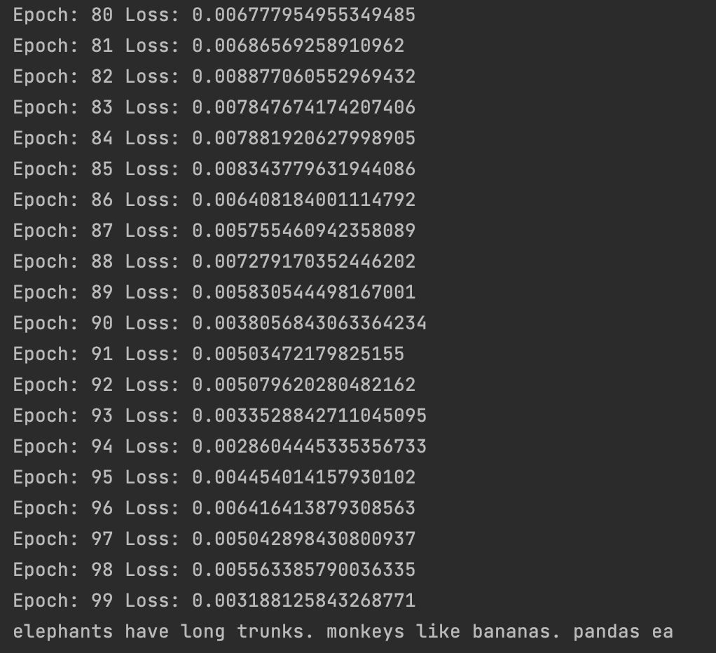
Of course, when training on such a small dataset the model will completely overfit it and learn to reproduce the whole dataset. Not what you are usually looking for in a language model, but in this "hello world" test it means success!
Saving and loading the model
Once you trained the model, it is useful if you can save it, so you don't have to train a new model every time.
To do this we add the following code to the LanguageModel class.
def save_checkpoint(self, path):
    print(f'Saving checkpoint {path}')
    torch.save({
        'number_of_tokens': self.number_of_tokens,
        'max_sequence_length': self.max_sequence_length,
        'embedding_dimension': self.embedding_dimension,
        'number_of_layers': self.number_of_layers,
        'number_of_heads': self.number_of_heads,
        'feed_forward_dimension': self.feed_forward_dimension,
        'dropout_rate': self.dropout_rate,
        'model_state_dict': self.state_dict()
    }, path)

@staticmethod
def load_checkpoint(path) -> 'LanguageModel':
    checkpoint = torch.load(path)
    model = LanguageModel(
        number_of_tokens=checkpoint['number_of_tokens'],
        max_sequence_length=checkpoint['max_sequence_length'],
        embedding_dimension=checkpoint['embedding_dimension'],
        number_of_layers=checkpoint['number_of_layers'],
        number_of_heads=checkpoint['number_of_heads'],
        feed_forward_dimension=checkpoint['feed_forward_dimension'],
        dropout_rate=checkpoint['dropout_rate']
    )
    model.load_state_dict(checkpoint['model_state_dict'])
    return model
Since we use the AutoregressiveWrapper as convenience class, we can give this wrapper the save and load methods too.
def save_checkpoint(self, path):
    self.model.save_checkpoint(path)

@staticmethod
def load_checkpoint(path) -> 'AutoregressiveWrapper':
    model = LanguageModel.load_checkpoint(path)
    return AutoregressiveWrapper(model)
This makes it possible to easily save and load a trained model using.
model.save_checkpoint('./trained_model')
model = model.load_checkpoint('./trained_model')
Running on GPU
If you have a GPU at your disposal and CUDA is configured, you can use a GPU to speed up training.
First we need to define a function to determine if we can use a GPU:
def get_device():
    if torch.cuda.is_available():
        return torch.device('cuda')
    else:
        return torch.device('cpu')
Then we need to move the model and all input tensors to our device. We can do this by using the torch function to.
When creating the model, move it to the device:
model = AutoregressiveWrapper(LanguageModel(
    embedding_dimension=embedding_dimension,
    number_of_tokens=number_of_tokens,
    number_of_heads=4,
    number_of_layers=3,
    dropout_rate=0.1,
    max_sequence_length=max_sequence_length
)).to(get_device())
In the Trainer.train method, move the input tensors and target to the device:
model_output, target = self.model.forward(
    x=input_tensor.to(get_device()),
    mask=mask_tensor.to(get_device())
)

loss = self.loss_function(model_output.transpose(1, 2), target.to(get_device()))
In the Generator.generate method, move the input tensor to the device:
input_tensor = torch.tensor(
    pad_left(
        sequence=start_tokens,
        final_length=self.model.max_sequence_length + 1,
        padding_token=padding_token
    ),
    dtype=torch.long
).to(get_device())
Note that we also use register_buffer for the positional encoding matrix in the PositionalEncoding class. This ensures that the precomputed positional encodings automatically move to the correct device along with the model, avoiding device mismatch errors.
The speedup achieved by using a GPU can be really significant.
Conclusion
While writing this blogpost I learned a lot about how the transformer works, and how we can use it to generate text. I hope you enjoyed reading it, and learned something new too!
Feel free to leave a comment if you have remarks, questions or just want to let me know what you think :)
The code for this blogpost is available at https://github.com/wingedsheep/transformer
Sources
Some resources that were incredibly helpful in helping me understand attention, the transformer architecture and GPT models.
- Attention is all you need by Ashish Vaswani, Noam Shazeer, Niki Parmar, Jakob Uszkoreit, Llion Jones, Aidan N. Gomez, Lukasz Kaiser, Illia Polosukhin https://arxiv.org/abs/1706.03762
- Transformer implementation by Phil Wang (Lucidrains) https://github.com/lucidrains/x-transformers
- The illustrated transformer by Jay Alammar https://jalammar.github.io/illustrated-transformer/
- Illustrated GPT-2 by Jay Alammar https://jalammar.github.io/illustrated-gpt2/
- MinGPT by Andrej Karpathy https://github.com/karpathy/minGPT
- Seq2seq and attention by Lena Voita https://lena-voita.github.io/nlp_course/seq2seq_and_attention.html
- The GPT-3 Architecture, on a Napkin by Daniel Dugas https://dugas.ch/artificial_curiosity/GPT_architecture.html