In Februari 2015 the artificial intelligence company DeepMind published an article in Nature showing they can solve a number of Atari games using Deep Q learning. The amazing part of this is that they didn't create a compact representation of the state of the games. They trained their algorithm purely on the pixels visible on screen and a score. Using this approach they get a better result than all the previous algorithms available, and manage to play 49 out of the 57 games to at least the level of a professional human game tester.
Since reading about their result I have been tinkering around with reinforcement learning. I managed to create some working implementations, but they were never very stable. They learned how to solve a problem, but then after some more training they would oscillate out of control and end up having to learn everything again. An infinite cycle of success and failure. This time I set the challenge for myself to solve the problem, but to also solve it in a way that can maintain its results; A robust deep Q learning algorithm.
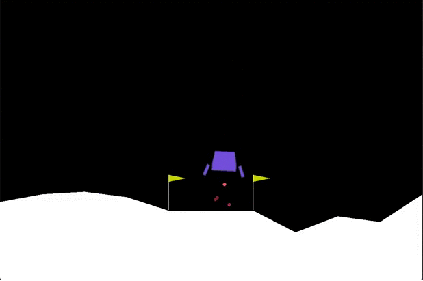
OpenAI created a platform for testing reinforcement learning agents. It contains implementations of different problems for reinforcement learning agents to solve, from simple grid worlds to more complex control problems. The goal for this blogpost is to solve the LunarLander-v2 environment.
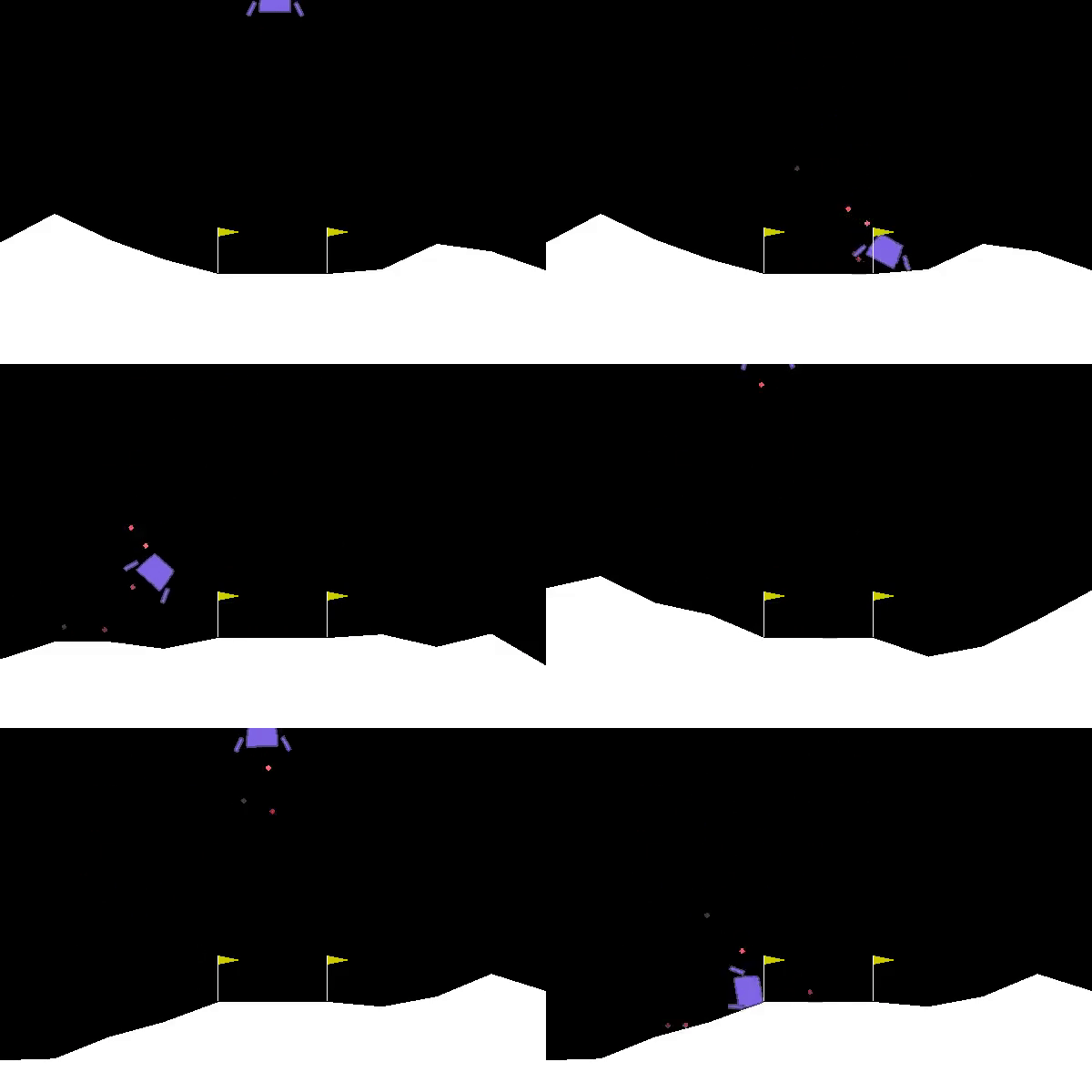
The goal of lunar lander is to land a small spacecraft between two flags. At every time step you have a choice between 4 actions: fire your main engine, your left engine, your right engine or do nothing. If the spacecraft hits the ground at the wrong angle or too fast it crashes and you get a large penalty. You also get a small penalty for firing your main engine. You get rewards for getting closer to the desired end position, and for touching the ground.
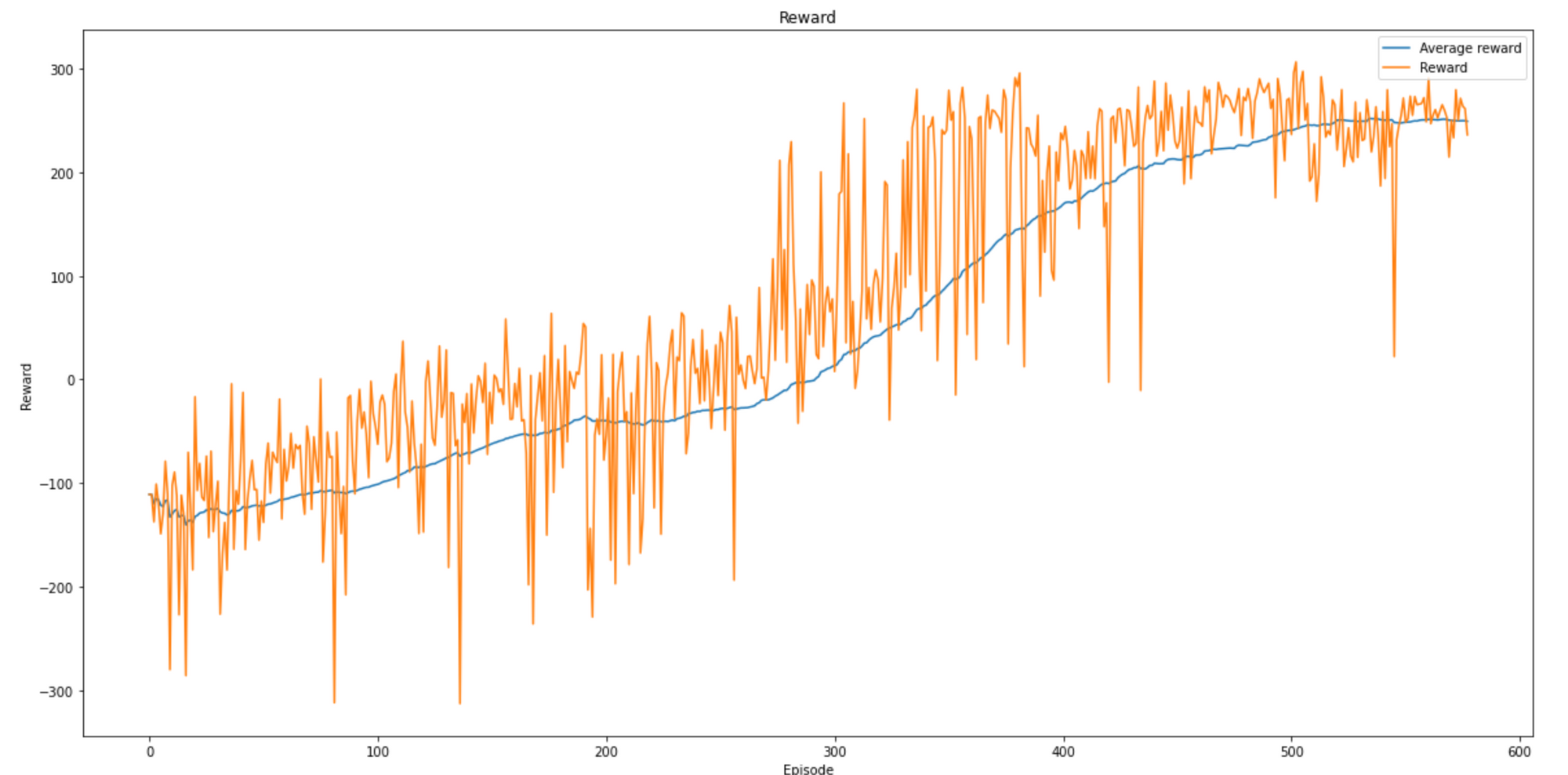
The environment is considered solved if the agent manages to get a score of 200 or more on average in the last 100 episodes.
Q learning
Let's first start by explaining a bit about the algorithm I am going to use. Q-learning is a reinforcement learning algorithm. In reinforcement learning an agent exists inside an environment. At every time step the agent can observe the environment and take an action. After taking an action the environment changes and the agent can observe the new state of the environment. In every transition from one state to another the agent receives feedback in the form of a reward or a penalty.
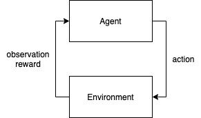
Q learning is an implementation of a reinforcement learning agent that learns about the environment and tries to maximize the expected reward gained.
It does this by using a Q-function Q(s, a).
Q(s, a) is a function that predicts the future reward in state s when taking action a. If your model is accurately predicting these Q values the agent could pick the action with the highest Q value to maximize its reward.
Usually in Q learning an agent begins by randomly selecting actions and observing their effects in the environment. It then uses the Bellman equation to update the Q function. The Bellman equation looks like this:

The agent was in state s and executed action a, it then ended up in state s' and received reward r. We then update the predicted value Q(s, a) by adjusting the current value with the temporal difference. The temporal difference can be described as the surprise of the reward you received. If the reward you received is higher than expected the temporal difference is positive, and if it is worse than expected the temporal difference is negative. If an action ended up to be better than expected we adjust the Q value upwards, and if it is worse than expected we adjust the Q value downwards.
The values explained in more detail:
- reward: the reward gained by moving from state s to state s' using action a.
- discount factor: how much to take the future into account. If the discount factor is 0 the future is not taken into account at all, if the discount factor is 1 we look an unlimited number of steps into the future. Say for instance the discount factor is 0.99, then we count an action 100 steps into the future only 0.99^100 = 0.366 times of the actual amount.
- learning rate: how much to adjust the Q function in every training step.
Practical example. Say we are in state s and the model predicted Q(s, a) to be 100. We then take action a and end up in state s'. We get a reward of 8. The Q value for the best action we could take in the next state s' is 95. A discount factor of 0.99 is used. We then get a temporal difference of: 8 + 0.99 * 95 - 100 = 2.05. We get 2.05 more reward from the action than expected. We don't want to adjust Q(s, a) to 102.5 right away, because making too large changes to the Q values might cause the model to never converge. So we update the model by the temporal difference multiplied by the learning rate, which is a value between 0 and 1. If the learning rate is 0.1 the new value for Q(s, a) becomes 100 + 0.1 * 2.05 = 100.205. The model is a bit more positive about selecting action a in state s.
The simplest implementation of Q-learning uses a table to hold all the values, but this quickly becomes infeasible for environments with many possible states or actions. By using a (deep) neural network to represent the Q(s, a) function the agent can generalise to never seen combinations of (s, a) better. The input for this neural network is an observation and the output is a Q value for every allowed action in that state. We call this implementation deep Q-learning.
Additions
Deep Q-learning can be quite unstable. Without any tweaks the algorithm can oscillate between good and bad solutions or fail to converge at all.
DeepMind used some additional tricks to make sure their deep Q-learning algorithm converges towards a good solution. In my implementation I am going to implement the following additions.
E-greedy action selection
Reinforcement learning is always a struggle between exploration and exploitation. If you always select the actions you think are the best (exploitation) you might never discover that there are better alternatives. If you explore too much you may never reach the better solutions.
I am going to implement e-greedy action selection. The idea of this method is to have a value between 0 and 1 that determines the amount of exploration vs exploitation. If the value is 0 the agent will always choose the action it thinks is the best one, if the value is 1 it will act completely random. The value starts out high and decreases over time. In the beginning the agent does not know anything about the environment, so it should explore as much to discover the effect of its actions on the environment. As the agent learns more it can start to exploit good strategies.
Experience replay
In the standard Q-learning algorithm the agent learns after every time step, all past experiences are thrown away.
With experience replay we save all state transitions (state, action, reward, new_state) so we can use them for training later.
The advantages of using experience replay are:
- You can use batches of state transitions to learn from. The model gets adjusted for a batch of transitions at once and makes sure that the update is beneficial for predicting each of these transitions. This leads to training updates that are good for multiple state / action pairs at the same time. This means more stable training and better convergence.
- You can revisit past states. Because there is a leaning rate, the model is not instantly adjusted to the correct values. It is nudged a bit in the right direction every training step. If you can revisit interesting actions you can learn more from them.
Double Q-learning
When calculating the target values for updating the model the same model is used for calculating Q(s, a) as for calculating the Q value of the best action in the next state. This can lead to overestimation of the expected reward.
For a detailed explanation read this blogpost by Rubik's code.
To solve this problem we use two models. The main model \( \theta \) for selecting actions and a target model \( \theta ' \) for calculating the target values. The weights of the main model are copied to the target model every x steps.
Vanilla target: \( R_{t+1} + \gamma max_{a}Q(S_{t+1}, a; \theta) \)
Double q learning target: \( R_{t+1} + \gamma Q(S_{t+1}, argmax_{a} Q(S_{t + 1}, a; \theta); \theta ') \)
\( Q(s, a; \theta) \) means the Q(s, a) value according to model \( \theta \), so the target is the reward plus the Q value of the target model with the best action in state the next state according to the main model.
Using double q learning leads to more realistic Q-values and thus to better models.
Huber loss
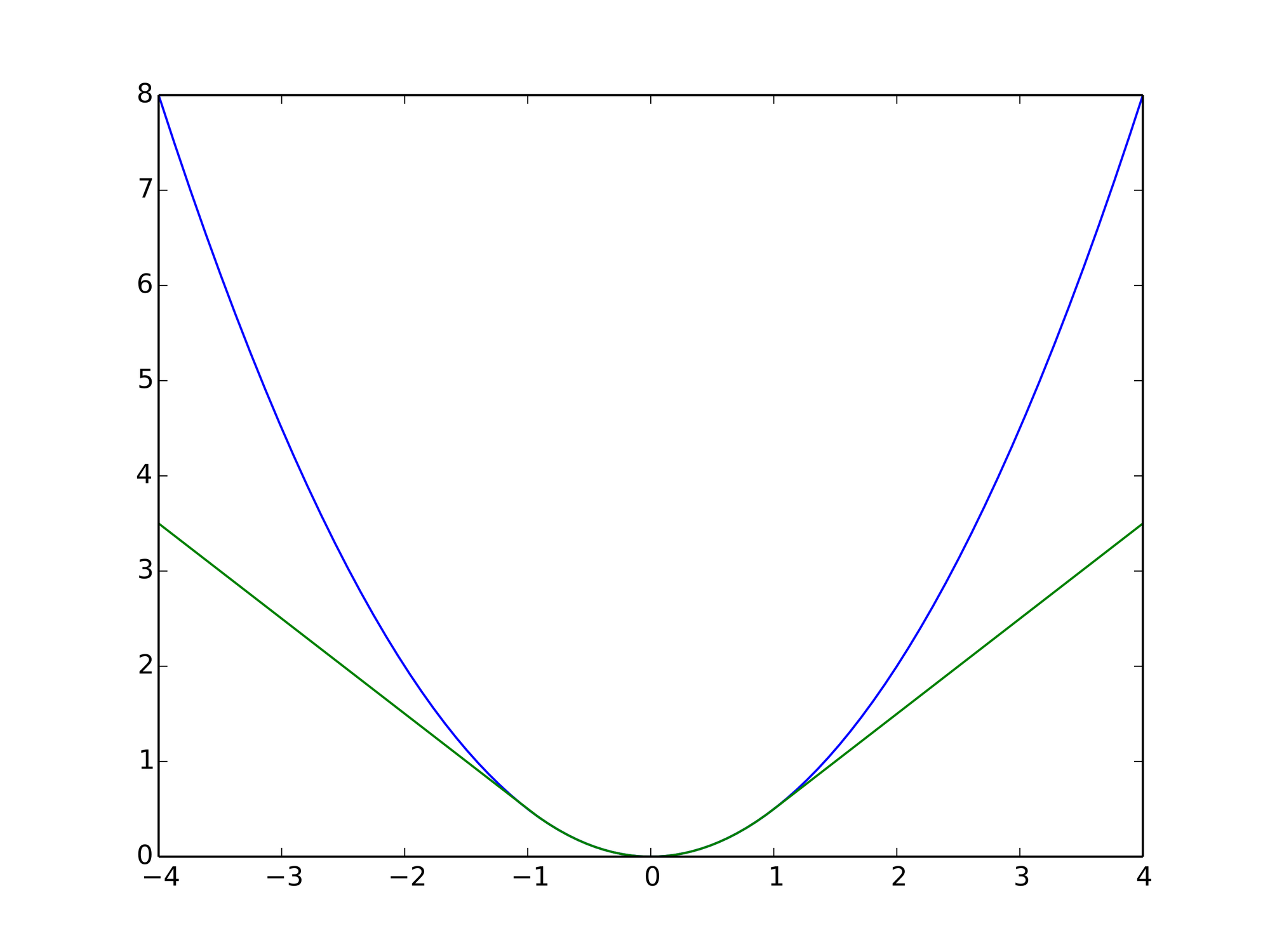
Using mean squared error (mse) as loss function might lead to very high errors when training. These high errors can cause the model to over-adjust and fail to converge to a good solution. Huber loss is less sensitive to outliers because it is exponential only up to a certain threshold and then becomes linear.
Using huber loss leads to a more stable Q-learning convergence.
Implementation
I implemented the algorithm on Google Colab where certain dependencies like Tensorflow come pre-installed. If you want to replicate this code on your local machine you will have to install some more dependencies than I show here.
First we are going to install box2d. This is necessary for running the LunarLander environment.
!pip install box2dThen we install the necessary modules.
import tensorflow as tf
import gym
import os
import random

from tensorflow.keras.models import Sequential, load_model
from tensorflow.keras.layers import Dense
from tensorflow.keras.regularizers import l2

import numpy as np
import scipy
import uuid
import shutil

import pandas as pd
import matplotlib.pyplot as plt
%matplotlib inline

import keras.backend as K
We create the LunarLander environment and check how large the state space and the action space are.
The state space describes the number of variables the agent can observe. Since we use observations as input for the Q-learning network this determines the number of inputs our model needs to have.
The action space describes how many actions are possible. For every action we are going to add an output to our Q-learning network.
env = gym.make("LunarLander-v2")

print(f"Input: {env.observation_space}")
print(f"Output: {env.action_space}")
It prints out the following. An observation contains 8 variables and we can choose between 4 different actions.
Input: Box(8,)
Output: Discrete(4)
Then we are going to create our model, but before we can do so we need to implement the Huber loss function. This might be the trickiest part of the implementation.
We implement this as a custom loss function using the Keras backend API. The function takes in all the predicted and true outputs for a batch of state transitions and has to calculate the average Huber loss over this batch. But there is a catch: Our model takes as input a state s, and as output the Q-values for all possible actions. If we want to update the model for a certain state transition (s, a, r, s') we only want to calculate the loss for the output that belongs to the action a that the agent took to get from state s to s'.
If we have four actions our model could predict [10, 13, 7, 9] as Q-values. In the state transition we are training on we took action 3 and got a target value of 12. We then get a target vector of [0, 0, 12, 0]. The masked_huber_loss function nullifies the error for outputs of which the y_true is 0. So the comparison becomes [0, 0, 7, 0] to [0, 0, 12, 0].
def masked_huber_loss(mask_value, clip_delta):
  def f(y_true, y_pred):
    error = y_true - y_pred
    cond  = K.abs(error) < clip_delta
    mask_true = K.cast(K.not_equal(y_true, mask_value), K.floatx())
    masked_squared_error = 0.5 * K.square(mask_true * (y_true - y_pred))
    linear_loss  = mask_true * (clip_delta * K.abs(error) - 0.5 * (clip_delta ** 2))
    huber_loss = tf.where(cond, masked_squared_error, linear_loss)
    return K.sum(huber_loss) / K.sum(mask_true)
  f.__name__ = 'masked_huber_loss'
  return f
We then create the model as follows. We have 9 input neurons. 8 for the observations in the LunarLander environment and 1 for the fraction complete. Fraction complete indicates how far the epsiode is to ending because of reaching its maximum number of steps. Say we have a maximum of 1000 steps and the current step is 400, then fraction complete is 0.4. This can be used by the agent to decide if it has to act fast, or if it can take it's time.
input_shape = (9,) # 8 variables in the environment + the fraction finished we add ourselves
outputs = 4

def create_model(learning_rate, regularization_factor):
  model = Sequential([
    Dense(64, input_shape=input_shape, activation="relu", kernel_regularizer=l2(regularization_factor)),
    Dense(64, activation="relu", kernel_regularizer=l2(regularization_factor)),
    Dense(64, activation="relu", kernel_regularizer=l2(regularization_factor)),
    Dense(outputs, activation='linear', kernel_regularizer=l2(regularization_factor))
  ])

  optimizer = tf.keras.optimizers.Adam(learning_rate=learning_rate)
  model.compile(optimizer=optimizer, loss=masked_huber_loss(0.0, 1.0))

  return model
We can use this model to predict Q-values for a single state or for a batch of states.
def get_q_values(model, state):
  input = state[np.newaxis, ...]
  return model.predict(input)[0]

def get_multiple_q_values(model, states):
  return model.predict(states)
These Q-values can be used to select actions. We use the epsilon greedy implementation like described above.
def select_action_epsilon_greedy(q_values, epsilon):
  random_value = random.uniform(0, 1)
  if random_value < epsilon:
    return random.randint(0, len(q_values) - 1)
  else:
    return np.argmax(q_values)

def select_best_action(q_values):
  return np.argmax(q_values)
Then we create the replay buffer with a certain size. If the number of state transitions in the replay buffer is bigger than the size it starts overwriting state transitions, starting from the oldest one. The replay buffer has a method to collect a batch of state transitions for training.
class StateTransition():

  def __init__(self, old_state, action, reward, new_state, done):
    self.old_state = old_state
    self.action = action
    self.reward = reward
    self.new_state = new_state
    self.done = done

class ReplayBuffer():
  current_index = 0

  def __init__(self, size = 10000):
    self.size = size
    self.transitions = []

  def add(self, transition):
    if len(self.transitions) < self.size:
      self.transitions.append(transition)
    else:
      self.transitions[self.current_index] = transition
      self.__increment_current_index()

  def length(self):
    return len(self.transitions)

  def get_batch(self, batch_size):
    return random.sample(self.transitions, batch_size)

  def __increment_current_index(self):
    self.current_index += 1
    if self.current_index >= self.size - 1:
      self.current_index = 0
When we want to train the model on a batch of state transitions we need to calculate the target values for each of these state / action pairs. We do this using the double Q-learning technique where we use two models for calculating the target values.
def calculate_target_values(model, target_model, state_transitions, discount_factor):
  states = []
  new_states = []
  for transition in state_transitions:
    states.append(transition.old_state)
    new_states.append(transition.new_state)

  new_states = np.array(new_states)

  q_values_new_state = get_multiple_q_values(model, new_states)
  q_values_new_state_target_model = get_multiple_q_values(target_model, new_states)

  targets = []
  for index, state_transition in enumerate(state_transitions):
    best_action = select_best_action(q_values_new_state[index])
    best_action_next_state_q_value = q_values_new_state_target_model[index][best_action]

    if state_transition.done:
      target_value = state_transition.reward
    else:
      target_value = state_transition.reward + discount_factor * best_action_next_state_q_value

    target_vector = [0] * outputs
    target_vector[state_transition.action] = target_value
    targets.append(target_vector)

  return np.array(targets)
We create a function to train the model using a batch of states and target values.
def train_model(model, states, targets):
  model.fit(states, targets, epochs=1, batch_size=len(targets), verbose=0)
Then we create a function to make a copy of a model. We need this later to create and update the target model. The model is saved to a backup file, which is loaded into a new object. The copy of the model is returned. We need to pass the masked_huber_loss to the load_model function, because Keras does not know how to initialize the new model otherwise. The backup just has a reference to the loss function name.
def copy_model(model):
  backup_file = 'backup_'+str(uuid.uuid4())
  model.save(backup_file)
  new_model = load_model(backup_file, custom_objects={ 'masked_huber_loss': masked_huber_loss(0.0, 1.0) })
  shutil.rmtree(backup_file)
  return new_model
Since we want to see how well the agent is learning we introduce some logging functionality. The AverageRewardTracker keeps count of the average reward over the last 100 steps. The FileLogger writes the results to a file after every episode.
class AverageRewardTracker():
  current_index = 0

  def __init__(self, num_rewards_for_average=100):
    self.num_rewards_for_average = num_rewards_for_average
    self.last_x_rewards = []

  def add(self, reward):
    if len(self.last_x_rewards) < self.num_rewards_for_average:
      self.last_x_rewards.append(reward)
    else:
      self.last_x_rewards[self.current_index] = reward
      self.__increment_current_index()

  def __increment_current_index(self):
    self.current_index += 1
    if self.current_index >= self.num_rewards_for_average:
      self.current_index = 0

  def get_average(self):
    return np.average(self.last_x_rewards)


class FileLogger():

  def __init__(self, file_name='progress.log'):
    self.file_name = file_name
    self.clean_progress_file()

  def log(self, episode, steps, reward, average_reward):
    f = open(self.file_name, 'a+')
    f.write(f"{episode};{steps};{reward};{average_reward}\n")
    f.close()

  def clean_progress_file(self):
    if os.path.exists(self.file_name):
      os.remove(self.file_name)
    f = open(self.file_name, 'a+')
    f.write("episode;steps;reward;average\n")
    f.close()
Then we define the hyperparameters.
replay_buffer_size = 200000
learning_rate = 0.001
regularization_factor = 0.001
training_batch_size = 128
training_start = 256
max_episodes = 10000
max_steps = 1000
target_network_replace_frequency_steps = 1000
model_backup_frequency_episodes = 100
starting_epsilon = 1.0
minimum_epsilon = 0.01
epsilon_decay_factor_per_episode = 0.995
discount_factor = 0.99
train_every_x_steps = 4
Finally it all comes together in the main loop.
replay_buffer = ReplayBuffer(replay_buffer_size)
model = create_model(learning_rate, regularization_factor)
target_model = copy_model(model)
epsilon = starting_epsilon
step_count = 0
average_reward_tracker = AverageRewardTracker(100)
file_logger = FileLogger()

for episode in range(max_episodes):
  print(f"Starting episode {episode} with epsilon {epsilon}")

  episode_reward = 0
  state = env.reset()
  fraction_finished = 0.0
  state = np.append(state, fraction_finished)

  first_q_values = get_q_values(model, state)
  print(f"Q values: {first_q_values}")
  print(f"Max Q: {max(first_q_values)}")

  for step in range(1, max_steps + 1):
    step_count += 1
    q_values = get_q_values(model, state)
    action = select_action_epsilon_greedy(q_values, epsilon)
    new_state, reward, done, info = env.step(action)

    fraction_finished = (step + 1) / max_steps
    new_state = np.append(new_state, fraction_finished)

    episode_reward += reward

    if step == max_steps:
      print(f"Episode reached the maximum number of steps. {max_steps}")
      done = True

    state_transition = StateTransition(state, action, reward, new_state, done)
    replay_buffer.add(state_transition)

    state = new_state

    if step_count % target_network_replace_frequency_steps == 0:
      print("Updating target model")
      target_model = copy_model(model)

    if replay_buffer.length() >= training_start and step_count % train_every_x_steps == 0:
      batch = replay_buffer.get_batch(batch_size=training_batch_size)
      targets = calculate_target_values(model, target_model, batch, discount_factor)
      states = np.array([state_transition.old_state for state_transition in batch])
      train_model(model, states, targets)

    if done:
      break

  average_reward_tracker.add(episode_reward)
  average = average_reward_tracker.get_average()

  print(
    f"episode {episode} finished in {step} steps with reward {episode_reward}. "
    f"Average reward over last 100: {average}")

  if episode != 0 and episode % model_backup_frequency_episodes == 0:
    backup_file = f"model_{episode}.h5"
    print(f"Backing up model to {backup_file}")
    model.save(backup_file)

  epsilon *= epsilon_decay_factor_per_episode
  epsilon = max(minimum_epsilon, epsilon)
When the training is done we can use the following code to visualise the training progress by loading the log file and plotting it using matplotlib.
data = pd.read_csv(file_logger.file_name, sep=';')

plt.figure(figsize=(20,10))
plt.plot(data['average'])
plt.plot(data['reward'])
plt.title('Reward')
plt.ylabel('Reward')
plt.xlabel('Episode')
plt.legend(['Average reward', 'Reward'], loc='upper right')
plt.show()
Results
After training the model for 578 steps I stopped training the model, because the model stopped improving. The average score over 100 episodes at that point was 248.97; a lot more than the required score of 200.0 to beat the environment.
Now it was time to see the model in action. To do this I loaded the last version of the model, turned off the training and rendered the results to the screen. It is actually working!
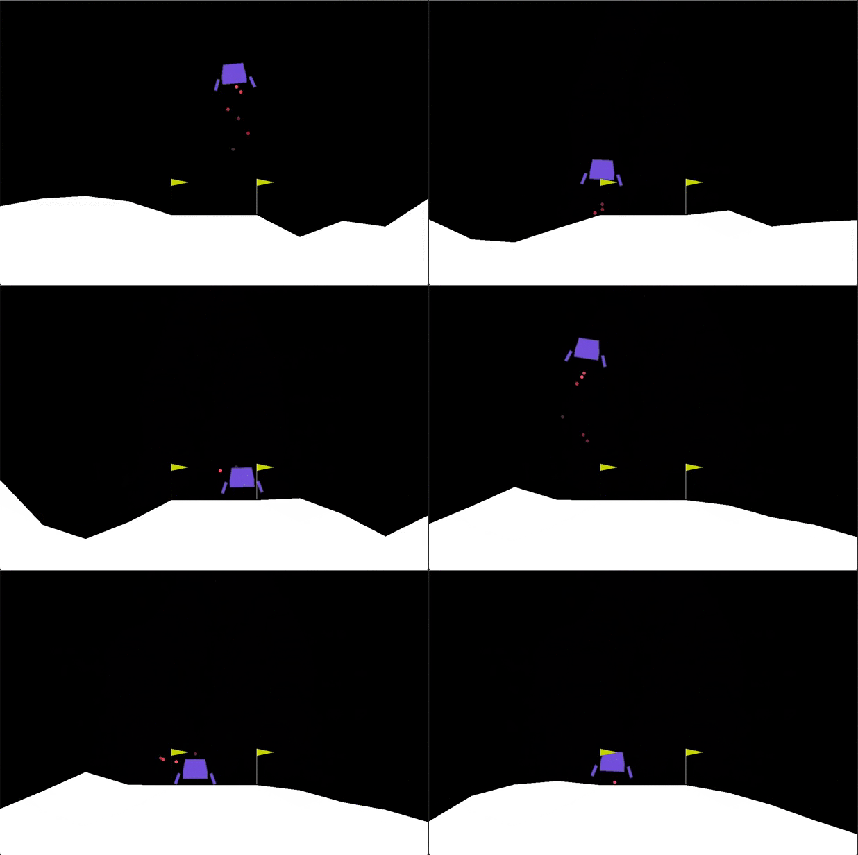
Although the model manages to get a pretty good score I still think it is quite slow at landing. In a future iteration of the algorithm I might add a penalty for taking too long.
Notes
2021-10-14: How to reproduce the visualisations?
I was asked a question about how to create the visualisations, and if they can be done in Colab. Here is my answer:
I didn't do the rendering on Google Colab, but on my local machine, because the OpenAI gym environment renders it in a window and this does not work in Colab.
Before you can run the script locally you need to have python and pip installed, and you need to install the following packages using "pip" https://pypi.org/project/pip/.
* gym: https://pypi.org/project/gym/
* tensorflow: https://pypi.org/project/tensorflow/
* numpy: https://pypi.org/project/numpy/
* box2d: https://pypi.org/project/box2d/
Here is a script that you can run locally to visualise runs of a certain model:
import gym
from tensorflow.keras.models import load_model
from tensorflow.keras.losses import MeanSquaredError
import numpy as np

env = gym.make("LunarLander-v2")
filename = "model_xxx.h5"
trained_model = load_model(filename, custom_objects={"masked_huber_loss": MeanSquaredError()})

evaluation_max_episodes = 10
evaluation_max_steps = 1000


def get_q_values(model, state):
    input = state[np.newaxis, ...]
    return model.predict(input)[0]


def select_best_action(q_values):
    return np.argmax(q_values)

rewards = []
for episode in range(1, evaluation_max_episodes + 1):
    state = env.reset()

    fraction_finished = 0.0
    state = np.append(state, fraction_finished)

    episode_reward = 0

    step = 1
    for step in range(1, evaluation_max_steps + 1):
        env.render()
        q_values = get_q_values(trained_model, state)
        action = select_best_action(q_values)
        new_state, reward, done, info = env.step(action)

        fraction_finished = (step + 1) / evaluation_max_steps
        new_state = np.append(new_state, fraction_finished)

        episode_reward += reward

        if step == evaluation_max_steps:
            print(f"Episode reached the maximum number of steps. {evaluation_max_steps}")
            done = True

        state = new_state

        if done:
            break

    print(f"episode {episode} finished in {step} steps with reward {episode_reward}.")
    rewards.append(episode_reward)

print("Average reward: " + np.average(rewards))
In the demo there is a line that says
filename = "model_xxx.h5"Here you can enter the name of the model you downloaded. If you look at the output of the Colab script you can see the models that are saved on the checkpoints. I updated the code in the blog to save the models as ".h5", which is the keras format for saving models. The advantage of this is that it is a single file that you can download from your Colab environment.
If you download a model you can put it in the same folder as the "lunarlander_demo.py" script, adjust the filename to point to and run the script.The environments of OpenAI have a "render()" function which renders the current state of the environment to the screen. This is used to render the runs.

